定积分比较大小
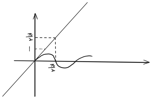
∫ 0 2 π x d x > ∫ 0 2 π sin x d x ∵ x > sin x ∴ ∫ 0 2 π x d x > ∫ 0 2 π sin x d x 图像法
比较∫ 0 1 x 2 d x ∫ 0 1 x 3 d x
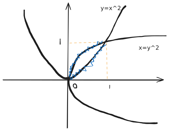
比较 [ 0 , 1 ] 内函数的大小 f ( x ) = x 2 f ( 2 1 ) = 4 1 g ( x ) = x 3 g ( 2 1 ) = 8 1 f ( x ) > g ( x ) ∴ ∫ 0 1 x 2 d x > ∫ 0 1 x 3 d x 比较∫ 0 1 x 2 d x ∫ 0 1 x d x
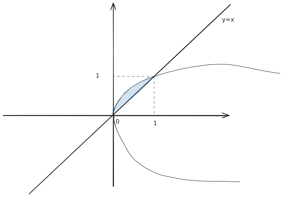
y = x y 2 = x ( 开口向右的抛物线 )
∴ ∫ 0 1 x 2 d x < ∫ 0 1 x d x 比较积分∫ 1 2 ln x d x ∫ 1 2 ( ln x ) 2 d x
当 1 ≤ x ≤ 2 , 0 = ln 1 ≤ ln x ≤ ln e = 1 即 0 ≤ ln x ≤ 1 我们知道当 0 ≤ u ≤ 1 , u 2 ≤ u 而 u > 1 时, u 2 > u ∴ ln x ≥ ( ln x ) 2 ,仅在 x = 1 处成立 ∴ ∫ 1 2 ln x d x > ∫ 1 2 ( ln x ) 2 d x 定积分性质
设f(x)在[a,b]上连续,下列不正确的是∫ 0 x f ( t ) d t
看∫ 0 x f ( t ) d t f ( t )
( ∫ 0 x f ( t ) d t ) ′ = f ( x ) ⋅ 1 = f ( x ) 所以正确
B.∫ x b f ( t ) d t − f ( x )
( ∫ x b f ( t ) d t ) ′ = f ( b ) ⋅ b ′ − f ( x ) = − f ( x ) 所以正确
C.∫ a b f ( x ) d x f ( x )
∫ a b f ( x ) d x 错误答案选C。
D.f ( x ) [a,b]上可积
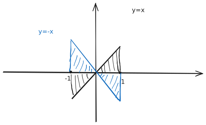
判断这句话是否正确,若在[a,b]上f(x),g(x)均连续且f ( x ) = g ( x ) ∫ a b f ( x ) d x = ∫ a b g ( x ) d x 令 a = − 1 , b = 1 , f ( x ) = x , g ( x ) = − x ∫ − 1 1 x d x 与 ∫ − 1 1 − x d x
如果在区间[a,b]上
g ( x ) = h ( x ) ( ∀ x ∈ [ a , b ]) 如果函数g(x),h(x)可积,那么
∫ a b g ( x ) d x = ∫ a b h ( x ) d x 设f(x)在区间[a,b]可积,且f(x)=1
∫ a b 1 d x = b − a 证明: x a b = b − a 设f(x)在区间[a,b]可积
∫ a b f ( x ) d x = − ∫ b a f ( x ) d x 证明: − ∫ b a f ( x ) d x = − [ F ( a ) − F ( b )] = F ( b ) − F ( a ) 如何估值
估计∫ 0 1 e x 2 d x
0 < x < 1 0 < x 2 < 1 e 0 < e x 2 < e 1 1 < e x 2 < e 两边同取定积分 ∫ 0 1 1 d x < ∫ 0 1 e x 2 < ∫ 0 1 e d x x 0 1 < ∫ 0 1 e x 2 < e x 0 1 1 < ∫ 0 1 e x 2 < e 估计定积分∫ − 1 1 e − x d x
− 1 < x < 1 1 > − x > − 1 − 1 < − x < 1 e − 1 < e − x < e ∫ − 1 1 e − 1 d x < ∫ − 1 1 e − x < ∫ − 1 1 e d x e − 1 x − 1 1 < ∫ − 1 1 e − x < e x − 1 1 e − 1 x − 1 1 = e − 1 − ( − 1 ) ⋅ e − 1 = 2 e − 1 e x − 1 1 = e − ( − e ) = 2 e ∴ e 2 < ∫ − 1 1 e − x < 2 e 估值定理
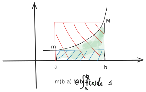
估值定理:如果f(x)在[a,b]上的最大值为M,最小值为m ,那么
m ( b − a ) ≤ ∫ a b f ( x ) d x ≤ M ( b − a ) 证明:
m ≤ f ( x ) ≤ M ∫ a b m d x ≤ ∫ a b f ( x ) d x ≤ ∫ a b M d x m ∫ a b d x ≤ ∫ a b f ( x ) d x ≤ M ∫ a b d x m x a b ≤ ∫ a b f ( x ) d x ≤ M x a b m ( b − a ) ≤ ∫ a b f ( x ) d x ≤ M ( b − a ) 另一种方法,用导数判断单调性,结合估值定理
令 f ( x ) = e − x f ′ ( x ) = − e − x < 0 ∴ f ( x ) 在 [ − 1 , 1 ] 单调递减 f ( x ) ma x = f ( x ) − 1 = e − ( − 1 ) = e f ( x ) min = f ( x ) 1 = e − 1 = e 1 根据估值定理 e 1 ⋅ ( 1 − ( − 1 )) ≤ ∫ − 1 1 e − x d x ≤ e ( 1 − ( − 1 )) e 2 ≤ ∫ − 1 1 e − x d x ≤ 2 e 估计积分∫ 4 π 4 3 π ( 1 + sin 2 x ) d x
令 f ( x ) = 1 + sin 2 x , x ∈ [ 4 π , 4 3 π ] f ′ ( x ) = 2 sin cos x = sin 2 x , x ∈ [ 4 π , 4 3 π ] 令 sin 2 x = 0 ⇒ 2 x = kπ ⇒ x = 2 kπ ∵ x ∈ [ 4 π , 4 3 π ] ∴ x = 2 π 为驻点 x [ 4 π , 2 π ] 2 π [ 2 π , 4 3 π ] f ′ ( x ) + 0 - f ( x ) 递增 极大值 递减 比较驻点,和端点值
f ( 2 π ) f ( 4 π ) f ( 4 3 π ) ∴ f ( x ) ma x f ( x ) min 根据估值定理 = 1 + ( sin 2 π ) 2 = 1 + 1 = 2 = 1 + ( sin 4 π ) 2 = 1 + ( 2 2 ) 2 = 1 + 2 1 = 2 3 = 1 + [ sin ( π − 4 π ) ] 2 = 1 + ( sin 4 π ) 2 = 2 3 = M = 2 = m = 2 3 m ⋅ ( 4 3 π − 4 π ) = 2 3 ⋅ 2 π = 4 3 π M ⋅ 2 π = 2 ⋅ 2 π = π ∴ 4 3 π ≤ ∫ 4 π 4 3 π ( 1 + sin 2 x ) d x ≤ π 积分中值定理
设f(x)在[a,b]上连续,则至少存在一点ξ ∈ [ a , b ] ξ ∈ ( a , b )
∫ a b f ( x ) d x = f ( ξ ) ( b − a )
Drawing 2026-01-06 18.27.41.excalidraw ⚠ Switch to EXCALIDRAW VIEW in the MORE OPTIONS menu of this document. ⚠ You can decompress Drawing data with the command palette: ‘Decompress current Excalidraw file’. For more info check in plugin settings under ‘Saving’
Excalidraw Data
Text Elements
a
b
Link to original f ( ξ ) = b − a 1 ∫ a b f ( x ) d x [a,b]上的平均值 。
证明:在估值定理的最后一步继续
m ≤ b − a ∫ a b f ( x ) d x ≤ M 由介值定理得,至少 ∃ ξ ∈ ( a , b ) ,使 f ( ξ ) = b − a ∫ a b f ( x ) d x 即 ∫ a b f ( x ) d x = f ( ξ ) ( b − a ) mean value theorem 介值定理
设f(x)在[0,2]上连续,f(0)=-1,2 1 ∫ 0 2 f ( x ) d x = 1 ∃ ξ ∈ ( 0 , 2 ) f ( ξ ) = 0
f ( x ) 在 [ 0 , 2 ] 上连续 由积分中职定理 ∃ ξ 1 ∈ ( 0 , 2 ) 使 ∫ 0 2 f ( x ) d x = 2 = 2 f ( ξ 1 ) 即 f ( ξ 1 ) = 1 又 ∵ f ( 0 ) = − 1 f ( 0 ) f ( ξ 1 ) < 0 由零点定理得至少存在一点 ξ ∈ ( 0 , 2 ) ,使 f ( ξ ) = 0 函数f ( x ) = 2 x + e 3 x [1,2]上的平均值 为?
2 − 1 1 ∫ 1 2 ( 2 x + e 3 x ) d x 2 ∫ 1 2 x d x + ∫ 1 2 e 3 x d x 2 ⋅ 2 x 2 1 2 + 3 1 e 3 x 1 2 3 + 3 1 e 6 − 3 1 e 3 求n项和极限
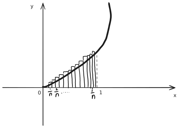
∫ 0 1 f ( x ) d x = n → ∞ lim [ f ( n 1 ) ⋅ n 1 + f ( n 2 ) ⋅ n 1 + f ( n 3 ) ⋅ n 1 + ⋯ f ( n i ) ⋅ n 1 + f ( n n ) ⋅ n 1 ] Sigma notation
n → ∞ lim [ f ( n 1 ) ⋅ n 1 + f ( n 2 ) ⋅ n 1 + f ( n 3 ) ⋅ n 1 + ⋯ f ( n i ) ⋅ n 1 + f ( n n ) ⋅ n 1 ] = n → ∞ lim i = 1 ∑ n f ( n i ) ⋅ n 1 n → ∞ lim n 1 ( 1 + n 1 + 1 + n 2 + … + 1 + n n ) 第一步写求和符号
i = 1 ∑ n 1 + n i 第二步找n i n 1
对 i 进行求和 , n 1 可以提出来 原式 = n → ∞ lim i = 1 ∑ n 1 + n i ⋅ n 1 第三步对应
n i → x n 1 → d x lim ∑ → ∫ n 1 < n i < n n 当 n → ∞ 0 < n i < 1 n → ∞ lim i = 1 ∑ n 1 + n i ⋅ n 1 = ∫ 0 1 1 + x d x n → ∞ lim n 2 1 ( n 2 − 1 2 + n 2 − 2 2 + ⋯ + n 2 − n 2 ) ( n 2 − 1 2 + n 2 − 2 2 + ⋯ + n 2 − n 2 ) = i = 1 ∑ n n 2 − i 2 原式 = n → ∞ lim n 2 1 i = 1 ∑ n n 2 − i 2 = n → ∞ lim n 1 i = 1 ∑ n n 2 − i 2 n 1 在这 i 和 n 齐次,考虑凑定积分定义 = n → ∞ lim i = 1 ∑ n n n 2 − i 2 n 1 = n → ∞ lim i = 1 ∑ n n 2 n 2 − i 2 n 1 = n → ∞ lim i = 1 ∑ n 1 − n 2 i 2 n 1 = n → ∞ lim i = 1 ∑ n 1 − ( n i ) 2 n 1 = ∫ 0 1 1 − x 2 d x i和n齐次,考虑凑定积分定义,如果非齐次考虑用夹逼定理。
n → ∞ lim ( n + 1 1 + n + 2 1 + ⋯ + n + n 1 ) n → ∞ lim i = 1 ∑ n n + i 1 n → ∞ lim i = 1 ∑ n n n + i n 1 n → ∞ lim i = 1 ∑ n 1 + n i 1 ⋅ n 1 = ∫ 0 1 1 + x 1 d x 对应技巧
n → ∞ lim i = 1 ∑ n n i sin n i ⋅ n 1 = ∫ 0 1 x sin x d x n → ∞ lim i = 1 ∑ 2 n n i sin n i ⋅ n 1 n 1 < n i < n 2 n ∴ 0 < n i < 2 n → ∞ lim i = 1 ∑ 2 n n i sin n i ⋅ n 1 = ∫ 0 2 x sin x d x n → ∞ lim i = 1 ∑ n f ( a + n i ) ⋅ n 1 看这个积分范围 0 < n i < 1 a < a + n i < 1 + a ∴ n → ∞ lim i = 1 ∑ n f ( a + n i ) ⋅ n 1 = ∫ a a + 1 f ( x ) d x n → ∞ lim i = 1 ∑ n ( 1 + n i ) 2 ⋅ n 1 = ∫ 1 2 x 2 d x = ∫ 0 1 ( 1 + x ) 2 d x 牛顿-莱布尼兹公式
如果函数F(x)是连续函数 f(x)在区间[a,b]上的一个原函数,则:
∫ a b f ( x ) d x = F ( x ) a b = F ( b ) − F ( a ) ∫ 1 2 x d x = 2 1 x 2 1 2 = 2 1 ⋅ 2 2 − 2 1 ⋅ 1 2 = 2 3 分部积分公式
∫ a b u v ′ d x = ∫ a b u d v = uv a b − ∫ a b v ⋅ u ′ d x 如:
∫ 0 1 x e x d x = ∫ 0 1 x d e x = x e x 0 1 − ∫ 0 1 e x d x = 1 ⋅ e − 0 − e x 0 1 = e − ( e − 1 ) = 1 例题
∫ 0 π t sin t d t − ∫ 0 π t d ( cos t ) − ( t ⋅ cos t 0 π − ∫ 0 π cos t d t ) − t ⋅ cos t 0 π + sin t 0 π π + 0 = π 换元法
定积分换元记得换限
∫ 1 4 x ( 1 + x ) 1 d x 换元,令 t = x , x = t 2 , d x = d t 2 = 2 t d t 上下限换元代入 t = x 上限换元 x = 4 , t = 2 ; 下限换元 x = 1 , t = 1 ∫ 1 2 t 2 ( 1 + t ) 1 2 t d t 2 ∫ 1 2 t 2 ( 1 + t ) 1 t d t 2 ∫ 1 2 t ( 1 + t ) 1 d t 2 ∫ 1 2 t 1 − 1 + t 1 d t 2 ( ln ∣ t ∣ − ln ∣1 + t ∣ ) 1 2 2 ln ∣ 1 + t t ∣ 1 2 2 ln 3 2 − 2 ln 2 1 = 2 ln 3 4 ∫ 0 1 x 2 1 − x 2 d x 令 x = sin t , d x = d sin t = cos t d t 上下限换元代入 x = sin t x = 1 , t = 2 π , x = 0 , t = 0 原式 = ∫ 0 2 π sin 2 t cos t ⋅ cos t d t ∫ 0 2 π sin 2 t cos 2 t d t ∫ 0 2 π ( 1 − cos 2 t ) ⋅ cos 2 t d t ∫ 0 2 π cos 2 t − cos 4 t d t 2 1 ⋅ 2 π − 4 3 ⋅ 2 1 ⋅ 2 π = 4 π − 16 3 π = 16 π 变限积分求导
形如:∫ g ( x ) f ( x ) h ( t ) d t ∫ 0 x 2 t d t , ∫ x x 2 2 t 3 d t
求导方法
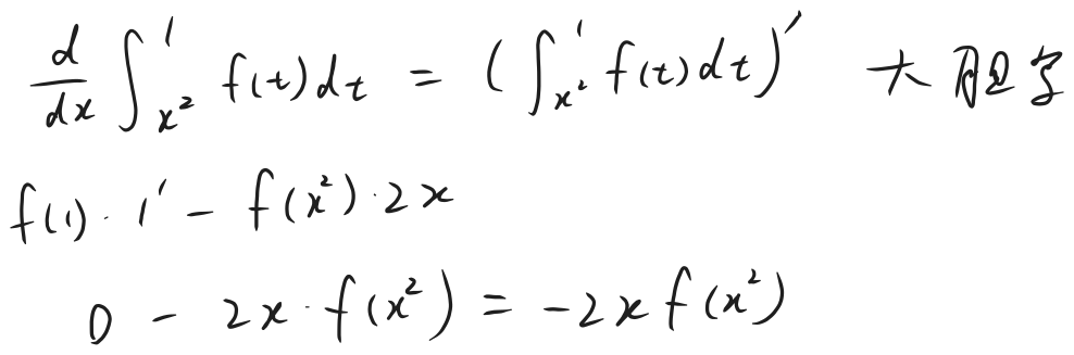
[ ∫ 下限 上限 f ( t ) d t ] ′ = f ( 上限 ) ⋅ 上 限 ′ − f ( 下限 ) ⋅ 下 限 ′ 做题中,遇到变限积分基本上就考求导
在极限中⇒
等式(结合微分方程)
求( ∫ 0 x 2 t 2 d t ) ′
( ∫ 0 x 2 t 2 d t ) ′ = 2 x 2 ⋅ ( x ) ′ − 2 ⋅ 0 2 = 2 x 2 设ϕ ( x ) = ∫ 0 x x cos t 2 d t ϕ ′ ( x )
常数因子可以拿到外面去,这道题是对t积分x就是常数因子,这个方法是对此积分类型先积分后求导的简便方法所以x可外提,即∫ a b k f ( x ) d x = k ∫ a b f ( x ) d x ( k 与 x 无关 )
∫ 0 x x cos t 2 d t = x ∫ 0 x cos t 2 d t ϕ ( x ) = x ∫ 0 x cos t 2 d t ϕ ′ ( x ) = ( x ) ′ ∫ 0 x cos t 2 d t + x ( ∫ 0 x cos t 2 d t ) ′ = ∫ 0 x cos t 2 d t + x ( cos x 2 − 0 ) = ∫ 0 x cos t 2 d t + x cos x 2 当 b = a 时 , ∫ a a f ( x ) d x = 0 求极限lim x → 0 ( e x − 1 ) t a n x ∫ 0 x s i n t d t
x → 0 lim ( e x − 1 ) tan x ∫ 0 x sin t d t = x → 0 lim x ⋅ x ∫ 0 x sin t d t x → 0 lim 2 x sin x = x → 0 lim 2 x x = 2 1 教材上的公式:
( ∫ ϕ ( x ) g ( x ) f ( t ) d t ) ′ = g ′ ( x ) f [ g ( x )] − ϕ ′ ( x ) f [ ϕ ( x )] 计算
[ ∫ 0 x e − t sin t ] ′ = 1 ⋅ e − x sin x = e − x sin x 已知F ( x ) = ∫ x 0 cos ( 3 t + 1 ) d t , 求 F ′ ( x )
F ′ ( x ) = 0 − cos ( 3 x + 1 ) ⋅ 1 = − cos ( 3 x + 1 ) 第二种解法 F ( x ) = ∫ x 0 cos ( 3 t + 1 ) d t = − ∫ 0 x cos ( 3 t + 1 ) d t ∴ F ′ ( x ) = − cos ( 3 x + 1 ) 设y = ∫ 1 x 2 1 + t 3 d t ,求 d x d y
d x d y = [ ∫ 1 x 2 1 + t 3 d t ] ′ = 1 + ( x 2 ) 3 ⋅ ( x 2 ) ′ − ( 1 ) ′ = 2 x 1 + x 6 求极限
x → 0 lim sin 2 x ∫ 0 2 x 2 e t 2 d t 第一步先带入,分子 ∫ 0 0 f ( t ) d t 趋于 0 分母也趋于 0 x → 0 lim x 2 ∫ 0 2 x 2 e t 2 d t 洛 x → 0 lim 2 x e ( 2 x 2 ) 2 ⋅ 4 x x → 0 lim 2 e 4 x 4 = 2
积分里含有x
取出x,再求导
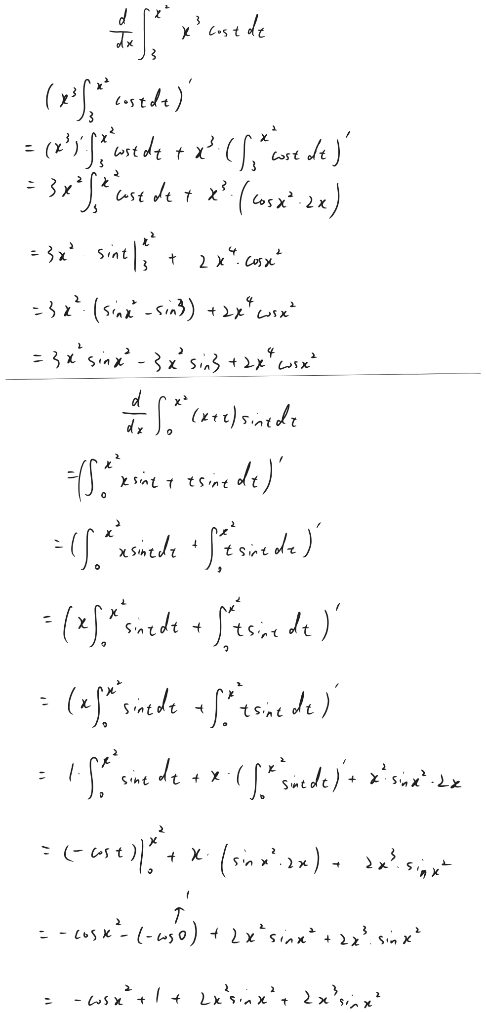
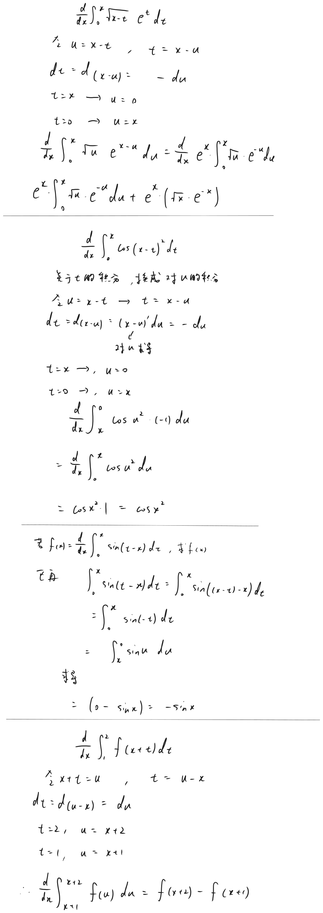
d x d ∫ 1 x 2 x e t d t = ( ∫ 1 x 2 x e t d t ) ′ 对 t 进行积分, x 当作常数 ( x ⋅ ∫ 1 x 2 e t d t ) ′ x ′ ⋅ ∫ 1 x 2 e t d t + x ⋅ ( ∫ 1 x 2 e t d t ) ′ 1 ⋅ ∫ 1 x 2 e t d t + x ⋅ ( e x 2 ⋅ 2 x ) = ∫ 1 x 2 e t d t + 2 x 2 e x 2 = e t 1 x 2 + 2 x 2 e x 2 = e x 2 − e + 2 x 2 e x 2
运算技巧
偶倍奇零
条件:区间对称
∫ − a a f ( x ) d x = { 2 ∫ 0 a f ( x ) d x , 0 , f ( x ) 为偶函数 f ( x ) 为奇函数 另一种情况,这里f ( x )
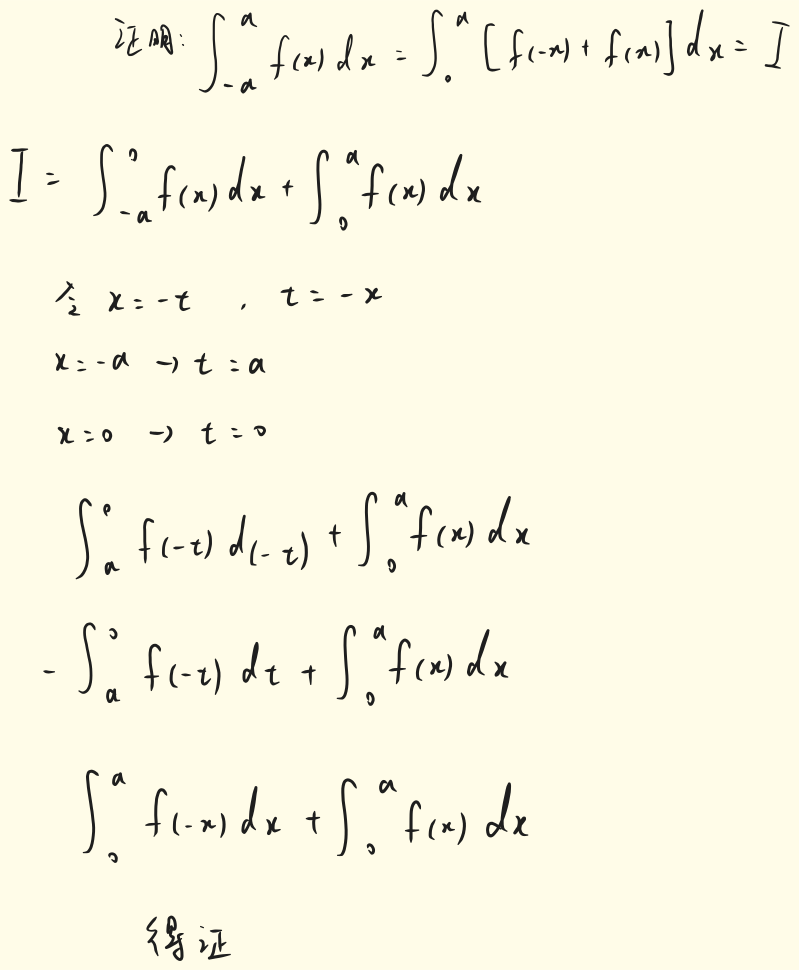
∫ − a a f ( x ) d x = ∫ 0 a [ f ( x ) + f ( − x )] d x 证明:
非奇非偶的处理
∫ − a a f ( x ) d x = ∫ 0 a f ( x ) + f ( − x ) d x Proof:
∫ − a a f ( x ) d x = ∫ − a 0 f ( x ) d x + ∫ 0 a f ( x ) d x Let x = − t , d x = − d t When x = − a , t = a ; x = 0 , t = 0 Now ∫ − a 0 f ( x ) d x = − ∫ a 0 f ( − t ) d t = ∫ 0 a f ( − x ) d x So ∫ − a a f ( x ) d x = ∫ 0 a f ( − x ) d x + ∫ 0 a f ( x ) d x Proof completed 题目
求∫ − 1 1 ( x 3 cos x + 1 ) d x
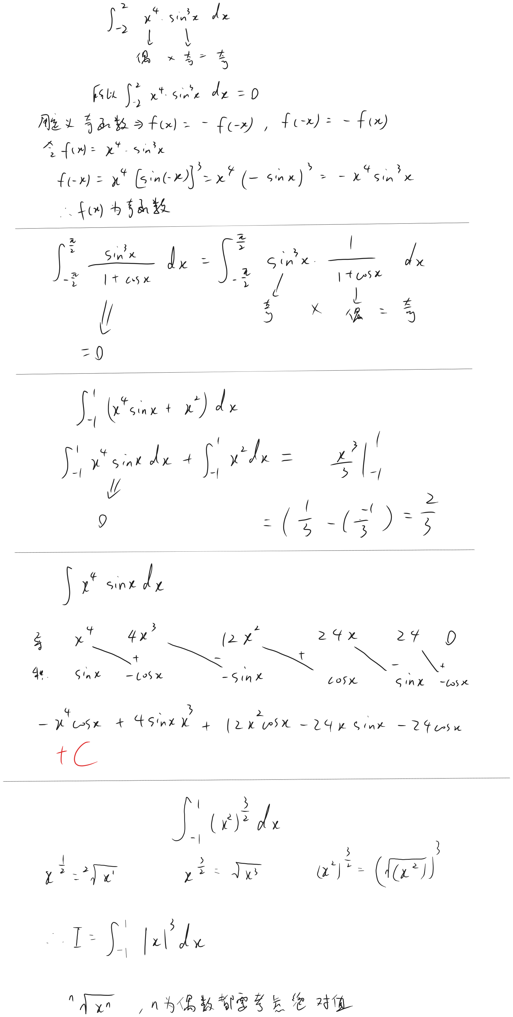
∫ − 1 1 ( x 3 cos x + 1 ) d x = ∫ − 1 1 x 3 cos x d x + ∫ − 1 1 1 d x x 3 奇函数 乘上 cos x 偶函数 = 奇函数 原式 = ∫ − 1 1 1 d x = x − 1 1 = 1 − ( − 1 ) = 2 因为1也是偶函数,也可用偶倍奇零
∫ − 1 1 1 d x = 2 ∫ 0 1 1 d x = 2 x 0 1 = 2 设f(x)在[-l,l]上连续,则 ∫ − l l f ( x ) − f ( − x ) d x =
令 F ( x ) F ( − x ) = f ( x ) − f ( − x ) = f ( − x ) − f ( x ) = − [ f ( x ) − f ( − x )] ∴ F ( x ) 为奇函数 ∫ − l l f ( x ) − f ( − x ) d x = 0 ∫ − 1 1 1 + x 2 2 + sin x d x = ∫ − 1 1 1 + x 2 2 d x + ∫ − 1 1 1 + x 2 sin x d x 其中 1 + x 2 2 , 2 偶函数, 1 偶函数, x 2 偶函数 1 + x 2 sin x , sin x 奇函数 2 ∫ − 1 1 1 + x 2 1 d x + 0 2 ⋅ 2 ∫ 0 1 1 + x 2 1 d x 4 arctan x 0 1 4 ( arctan 1 − arctan 0 ) 4 ⋅ 4 π = π arctan 1 tan多少度等于1
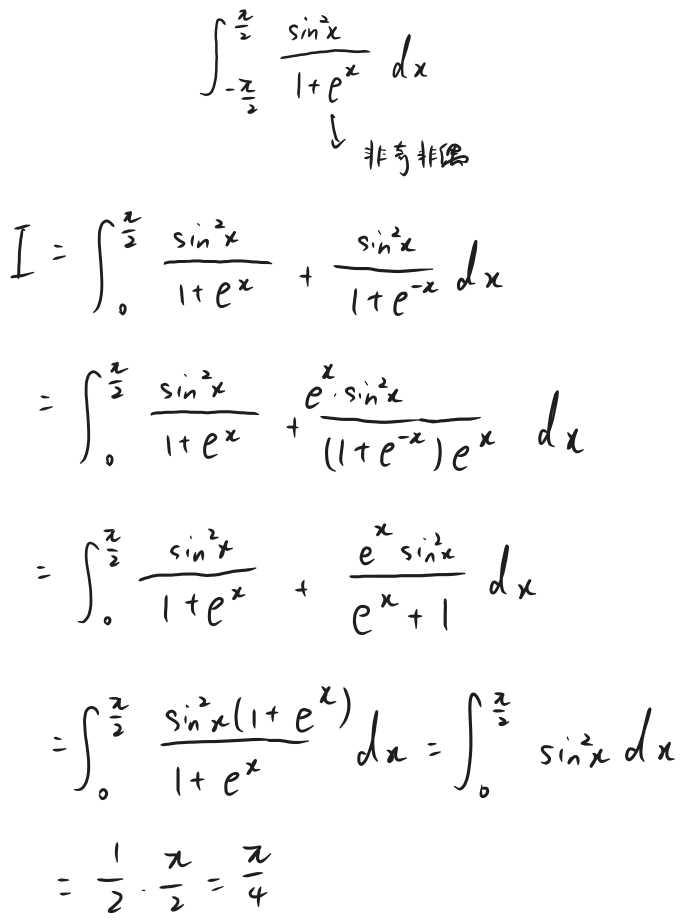
∫ − π π ( 1 + cos x + ∣ x ∣ ⋅ sin x ) d x cos 2 x = 2 cos 2 x − 1 cos 2 ⋅ 2 x = 2 cos 2 2 x − 1 ∫ − π π 1 + cos x d x + ∫ − π π ∣ x ∣ sin x d x cos x 偶函数, ∣ x ∣ 偶函数, sin x 奇函数 , 奇 × 偶 = 奇 2 ∫ 0 π 1 + cos x d x (消 1 ) 2 ∫ 0 π 1 + 2 cos 2 2 x − 1 d x 2 ∫ 0 π 2 cos 2 2 x d x x ∈ ( 0 , π ) , 2 x ∈ ( 0 , 2 π ) ∴ 2 ∫ 0 π 2 ⋅ cos 2 x d x 2 2 ∫ 0 π cos 2 x d x 4 2 ∫ 0 π cos 2 x d 2 x 4 2 sin 2 x 0 π = 4 2 sin 2 π = 4 2 求∫ − 1 1 e x 2 sin x d x f ( x ) = e x 2 sin x
f ( x ) = e ∣ x ∣ sin x 令 g ( x ) = e ∣ x ∣ g ( − x ) = e ∣ x ∣ ∴ e ∣ x ∣ 为偶函数 偶函数 × 奇函数 = 奇函数 ∴ ∫ − 1 1 e x 2 sin x d x = 0 另一种看法,用复合函数的奇偶行判断全奇则奇,遇偶则偶,e ∣ x ∣
∫ − 1 1 [ x 4 + 2 x 2 + 1 x 3 sin 2 x + ( x 2 + 1 ) 1 − x 2 ] d x x 3 奇 × sin 2 x 偶 = 奇 x 4 + 2 x 2 + 1 = 偶 奇 × 偶 = 奇 ∴ ∫ − 1 1 x 4 + 2 x 2 + 1 x 3 sin 2 x d x = 0 ∫ − 1 1 ( x 2 + 1 ) 1 − x 2 = 2 ∫ 0 1 ( x 2 + 1 ) 1 − x 2
Drawing 2026-03-10 16.49.37.excalidraw ⚠ Switch to EXCALIDRAW VIEW in the MORE OPTIONS menu of this document. ⚠ You can decompress Drawing data with the command palette: ‘Decompress current Excalidraw file’. For more info check in plugin settings under ‘Saving’
Excalidraw Data
Text Elements Link to original
华里氏公式
点火公式
∫ 0 2 π sin n x d x = ∫ 0 2 π cos n x d x = ⎩ ⎨ ⎧ n n − 1 ⋅ n − 2 n − 3 ⋅ n − 5 n − 4 ⋯ 2 1 ⋅ 2 π , n 为偶数 n n − 1 ⋅ n − 2 n − 3 ⋯ 3 2 ⋅ 1 , n 为奇数 ∫ 0 π sin n d x = 2 ∫ 0 2 π sin n x d x ∫ 0 2 π cos 6 x d x = 6 5 ⋅ 4 3 ⋅ 2 1 ⋅ 2 π ∫ 0 2 π sin 5 x d x = 5 4 ⋅ 3 2 ⋅ 1 ∫ − 2 π 2 π ( sin 4 θ + cos 3 θ ) d θ 对称区间优先用偶倍奇零
sin 4 θ ,奇(偶) = 偶函数, cos 3 θ ,偶(奇) = 偶函数 2 ∫ 0 2 π sin 4 θ + cos 3 θ d θ 2 ( 4 3 ⋅ 2 1 ⋅ 2 π + 3 2 ⋅ 1 ) = 8 3 π + 3 4
Drawing 2026-03-10 17.06.49.excalidraw ⚠ Switch to EXCALIDRAW VIEW in the MORE OPTIONS menu of this document. ⚠ You can decompress Drawing data with the command palette: ‘Decompress current Excalidraw file’. For more info check in plugin settings under ‘Saving’
Excalidraw Data
Text Elements Link to original
三角函数积分变换公式
设f(x)在[0,1]上连续,则
∫ 0 2 π f ( sin x ) d x = ∫ 0 2 π f ( cos x ) d x 可以用区间再现公式证明。
∫ 0 π f ( sin x ) d x = 2 ∫ 0 2 π f ( sin x ) d x 因为sinx的图像关于x = 2 π
∴ ∫ 0 π sin x d x = 2 ∫ 0 2 π sin x d x 因为一个函数本身关于一条竖线轴对称,在这个函数外面再套一层函数,整个复合函数也关于该对称轴对称。由此简单证明:∫ 0 π f ( sin x ) d x = 2 ∫ 0 2 π f ( sin x ) d x
严格证明:
Drawing 2026-03-09 18.08.49.excalidraw ⚠ Switch to EXCALIDRAW VIEW in the MORE OPTIONS menu of this document. ⚠ You can decompress Drawing data with the command palette: ‘Decompress current Excalidraw file’. For more info check in plugin settings under ‘Saving’
Excalidraw Data
Text Elements Link to original
带绝对值
当被积函数含有绝对值符号时,应用定积分的性质,把积分区间分成若干个子区间,这样就可以把绝对值符号去掉,然后分别在各个子区间求定积分
∫ − 1 1 x 2 d x = ∫ − 1 1 ∣ x ∣ d x ∫ − 1 0 − x d x + ∫ 0 1 x d x − 2 1 x 2 − 1 0 + 2 1 x 2 0 1 0 − ( − 2 1 ) + 2 1 = 1 这道题也可以先用偶倍奇零
= ∫ − 1 1 ∣ x ∣ d x = 2 ∫ 0 1 ∣ x ∣ d x = 2 ⋅ 2 1 x 2 0 1 = 2 ( 2 1 ) = 1 ∫ 0 π sin x − sin 3 x d x ∫ 0 π sin x ( 1 − sin 2 x ) d x ∫ 0 π sin x ∣ cos x ∣ d x ∫ 0 2 π sin x cos x d x + ∫ 2 π π sin x ⋅ ( − cos x ) d x ∫ 0 2 π sin x cos x d x − ∫ 2 π π sin x cos x d x ∫ 0 2 π sin x d sin x − ∫ 2 π π sin x d sin x 3 2 sin x 2 3 0 2 π − 3 2 sin x 2 3 2 π π 3 2 − ( 0 − ( 3 2 ) ) = 3 4 ∫ 0 2 π ∣ sin x ∣ d x i 第一种办法分区间讨论绝对值
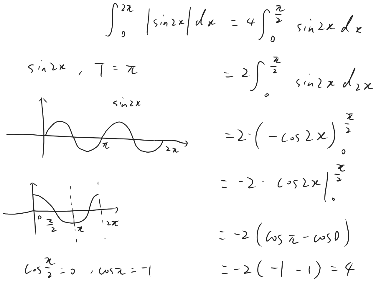
∫ 0 π sin x d x + ∫ π 2 π ( − sin x ) d x − cos x 0 π + cos x π 2 π − ( cos π − cos 0 ) + ( cos 2 π − cos π ) − ( − 1 − 1 ) + ( 1 − ( − 1 )) = 4 第二种办法,直接看∣ sin x ∣
Drawing 2026-01-07 16.44.47.excalidraw ⚠ Switch to EXCALIDRAW VIEW in the MORE OPTIONS menu of this document. ⚠ You can decompress Drawing data with the command palette: ‘Decompress current Excalidraw file’. For more info check in plugin settings under ‘Saving’
Excalidraw Data
Text Elements Link to original
∫ 0 2 π ∣ sin x ∣ d x = 2 ∫ 0 π sin x 2 ⋅ ( − cos x ) 0 π 2 ⋅ − ( cos π − cos 0 ) = − 2 ⋅ ( − 1 − 1 ) = 4
几何应用
求圆的面积
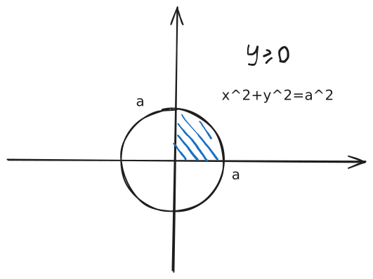
∫ 0 a a 2 − x 2 d x = 4 1 π a 2
∫ 0 2 4 − x 2 d x = ∫ 0 2 2 − x 2 d x = 4 1 π ⋅ 2 2 = π
∫ − a a ( b + x ) ⋅ a 2 − x 2 d x ∫ − a a b a 2 − x 2 + x a 2 − x 2 d x 令 f ( x ) = b a 2 − x 2 a 2 − x 2 ≥ 0 a 2 ≥ x 2 ∣ x ∣ 2 ≤ ∣ a ∣ 2 ∣ x ∣ ≤ ∣ a ∣ − ∣ a ∣ ≤ x ≤ ∣ a ∣ ∴ x ∈ [ − ∣ a ∣ , ∣ a ∣ ] 大于取两边,小于取中间
∣ x ∣ ≥ 6 x ≥ 6 或 x ≤ − 6 ∣ x ∣ ≤ 6 x ≥ − 6 或 x ≤ 6 x ∈ [ − ∣ a ∣ , ∣ a ∣ ] 定义域关于 0 对称,满足判断偶函数的前提条件 f ( x ) = b a 2 − x 2 f ( − x ) = b a 2 − x 2 ∴ f ( x ) 为偶函数 ∫ − a a b a 2 − x 2 + ∫ − a a x a 2 − x 2 d x x a 2 − x 2 , 奇 × 偶 = 奇 2 ∫ 0 a b a 2 − x 2 d x 2 b ∫ 0 a a 2 − x 2 d x 2 b ⋅ 4 1 π a 2 = 2 1 a 2 bπ 设f ( x ) = 3 x − 1 − x 2 − ∫ 0 1 f ( x ) d x f ( x ) ∫ 0 1 f ( x ) d x = A f ( x ) = 3 x − 1 − x 2 − A
∫ 0 1 f ( x ) d x A A 2 A A ∴ f ( x ) = ∫ 0 1 3 x d x − ∫ 0 1 1 − x 2 d x − ∫ 0 1 A d x = 3 ⋅ 2 1 x 2 0 1 − 4 1 π − A x 0 1 = 2 3 − 4 1 π − A = 2 3 − 4 1 π = 4 3 − 8 1 π = 3 x − 1 − x 2 − 4 3 + 8 π 用几何法求简单定积分
∫ − 2 2 4 − x 2 d x 令 y = 4 − x 2 y 2 = 4 − x 2 ( y ≥ 0 ) x 2 + y 2 = 2 2 ( y ≥ 0 ) 反映到几何上
Drawing 2025-12-24 14.39.02.excalidraw ⚠ Switch to EXCALIDRAW VIEW in the MORE OPTIONS menu of this document. ⚠ You can decompress Drawing data with the command palette: ‘Decompress current Excalidraw file’. For more info check in plugin settings under ‘Saving’
Excalidraw Data
Text Elements
2
-2
Link to original
∴ ∫ − 2 2 4 − x 2 d x = 2 1 π 2 2 = 2 π 求∫ − 1 1 1 − x 2 d x
令 y = 1 − x 2 ,在区间 [ − 1 , 1 ] 连续 y 2 = 1 − x 2 ( y ≥ 0 ) x 2 + y 2 = 1 ( y ≥ 0 )
Drawing 2025-12-24 14.39.02.excalidraw 1 ⚠ Switch to EXCALIDRAW VIEW in the MORE OPTIONS menu of this document. ⚠ You can decompress Drawing data with the command palette: ‘Decompress current Excalidraw file’. For more info check in plugin settings under ‘Saving’
Excalidraw Data
Text Elements
1
-1
Link to original
∫ − 1 1 1 − x 2 d x = 2 1 π 1 2 = 2 π ∫ − 1 1 x 2 d x = ∫ − 1 1 ∣ x ∣ d x
Drawing 2025-12-30 13.44.00.excalidraw ⚠ Switch to EXCALIDRAW VIEW in the MORE OPTIONS menu of this document. ⚠ You can decompress Drawing data with the command palette: ‘Decompress current Excalidraw file’. For more info check in plugin settings under ‘Saving’
Excalidraw Data
Text Elements
-1
1
x
y
y=|x|
Link to original
∴ ∫ − 1 1 x 2 d x = 2 ⋅ 2 1 ⋅ 1 ⋅ 1 = 1 直角坐标系内求所围面积
简单理解
X 型图:由上、下两个函数围成的面积(分上、下观看)Drawing 2026-01-08 09.30.14.excalidraw ⚠ Switch to EXCALIDRAW VIEW in the MORE OPTIONS menu of this document. ⚠ You can decompress Drawing data with the command palette: ‘Decompress current Excalidraw file’. For more info check in plugin settings under ‘Saving’
Excalidraw Data
Text Elements
a
b
上f(x)
下f(x)
Link to original
推导面积过程
S = ∫ a b f 上 ( x ) d x − ∫ a b f 下 ( x ) d x S = ∫ a b f 上 ( x ) − f 下 ( x ) d x
Y 型图:分左、右看;左边一个函数,右边一个函数Drawing 2026-01-08 09.35.38.excalidraw ⚠ Switch to EXCALIDRAW VIEW in the MORE OPTIONS menu of this document. ⚠ You can decompress Drawing data with the command palette: ‘Decompress current Excalidraw file’. For more info check in plugin settings under ‘Saving’
Excalidraw Data
Text Elements
y
x
左f(y)
右f(y)
c
d
Link to original
∫ c d f 右 ( y ) − f 左 ( y ) d y
选用 Y 型;改写为 x = f(y)
严谨理解
X 型:曲线y = f ( x ) x = a , x = b ( a < b )
Drawing 2026-01-08 09.42.17.excalidraw ⚠ Switch to EXCALIDRAW VIEW in the MORE OPTIONS menu of this document. ⚠ You can decompress Drawing data with the command palette: ‘Decompress current Excalidraw file’. For more info check in plugin settings under ‘Saving’
Excalidraw Data
Text Elements
b
a
x
y
o
Link to original
A = ∫ a b ∣ f ( x ) ∣ d x y = f ( x ) , y = g ( x ) x = a , x = b ( a < b )
Drawing 2026-01-08 09.48.38.excalidraw ⚠ Switch to EXCALIDRAW VIEW in the MORE OPTIONS menu of this document. ⚠ You can decompress Drawing data with the command palette: ‘Decompress current Excalidraw file’. For more info check in plugin settings under ‘Saving’
Excalidraw Data
Text Elements
a
b
x
y
o
f(x)
g(x)
Link to original
A = ∫ a b ∣ f ( x ) − g ( x ) ∣ d x
Y 型:曲线x = ϕ ( y ) y = c , y = d ( c < d )
Drawing 2026-01-08 09.54.15.excalidraw ⚠ Switch to EXCALIDRAW VIEW in the MORE OPTIONS menu of this document. ⚠ You can decompress Drawing data with the command palette: ‘Decompress current Excalidraw file’. For more info check in plugin settings under ‘Saving’
Excalidraw Data
Text Elements
c
d
Link to original
A = ∫ c d ∣ φ ( y ) ∣ d y
Y 型:曲线x = φ ( y ) , x = ψ ( y ) y = c , y = d ( c < d ) Drawing 2026-01-08 09.56.06.excalidraw ⚠ Switch to EXCALIDRAW VIEW in the MORE OPTIONS menu of this document. ⚠ You can decompress Drawing data with the command palette: ‘Decompress current Excalidraw file’. For more info check in plugin settings under ‘Saving’
Excalidraw Data
Text Elements
c
d
Link to original
A = ∫ c d ∣ φ ( y ) − ψ ( y ) ∣ d y 题目
定义
设y = f ( x ) y = g ( x ) [a,b]上连续,则由这两条曲线及x = a , x = b
Circular transclusion detected: Math/lib/Integral-libs/Drawing-2026-01-08-09.48.38.excalidraw
∴ S = ∫ a b ∣ f ( x ) − g ( x ) ∣ d x 求面积
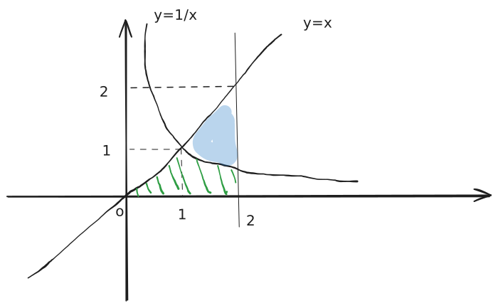
求y = x 2 , y = x 1 , x = 2
Drawing 2026-01-08 10.06.44.excalidraw ⚠ Switch to EXCALIDRAW VIEW in the MORE OPTIONS menu of this document. ⚠ You can decompress Drawing data with the command palette: ‘Decompress current Excalidraw file’. For more info check in plugin settings under ‘Saving’
Excalidraw Data
Text Elements
1
1
2
Link to original
画图后,发现用 X 型图比较好算
S = ∫ 1 2 ( x 2 − x 1 ) d x = [ 3 1 x 3 − ln ∣ x ∣ ] 1 2 = ( 3 8 − ln 2 ) − ( 3 1 − ln 1 ) = 3 7 − ln 2 或者用带绝对值的公式
S = ∫ 1 2 ∣ x 1 − x 2 ∣ d x 2 3 1 − ( 2 3 ) 2 = 3 2 − 4 9 < 0 去掉绝对值 S = ∫ 1 2 ( x 2 − x 1 ) d x 也是一样的 求y = x 2 , y = x
Drawing 2026-01-08 10.45.27.excalidraw ⚠ Switch to EXCALIDRAW VIEW in the MORE OPTIONS menu of this document. ⚠ You can decompress Drawing data with the command palette: ‘Decompress current Excalidraw file’. For more info check in plugin settings under ‘Saving’
Excalidraw Data
Text Elements
0
1
1
Link to original
{ y = x 2 y = x x 2 = x x 4 = x 可知交点坐标为 ( 0 , 0 ) 和 ( 1 , 1 ) ∴ S = ∫ 0 1 ( x − x 2 ) d x = ( 3 2 x 2 3 − 3 1 x 3 ) 0 1 = ( 3 2 − 3 1 ) = 3 1 也可以用Y型来做
Drawing 2026-01-08 10.45.27.excalidraw 1 ⚠ Switch to EXCALIDRAW VIEW in the MORE OPTIONS menu of this document. ⚠ You can decompress Drawing data with the command palette: ‘Decompress current Excalidraw file’. For more info check in plugin settings under ‘Saving’
Excalidraw Data
Text Elements
0
1
1
Link to original
y y ∴ S = x 2 ( y ≥ 0 ) ⇒ x = y ( y ≥ 0 ) = x ⇒ x = y 2 = ∫ 0 1 ( y − y 2 ) d y 求由曲线y = x 1 , y = x , x = 2
S = S 1 + S 2 S 1 = ∫ 0 1 x d x = 2 1 x 2 0 1 = 2 1 S 2 = ∫ 1 2 x 1 d x = ln ∣ x ∣ 1 2 = ln 2 − ln 1 = ln 2 ∴ S = 2 1 + ln 2 第二种方法,先求大三角形的面积,再减去旁边的阴影面积(蓝色)
S △ = ∫ 0 2 x d x = 2 1 x 2 0 2 = 2 S 阴 = ∫ 1 2 x d x − ∫ 1 2 x 1 d x = 2 1 x 2 1 2 − ln ∣ x ∣ 1 2 = 2 4 − 2 1 − ( ln 2 − ln 1 ) = 2 3 − ln 2 ∴ S = 2 − 2 3 + ln 2 = 2 1 + ln 2 求曲线x = y 2 y = x y 2 = x
{ y 2 = x y = x 交点 ( 0 , 0 ) 和 ( 1 , 1 ) y 2 = x ( x ≥ 0 ) y = x ( x ≥ 0 ) ∫ 0 1 x d x − ∫ 0 1 x d x = 3 2 x 2 3 0 1 − 2 1 x 2 0 1 = 3 2 − 2 1 = 6 4 − 6 3 = 1 求曲线y 2 = − x y 2 = − x
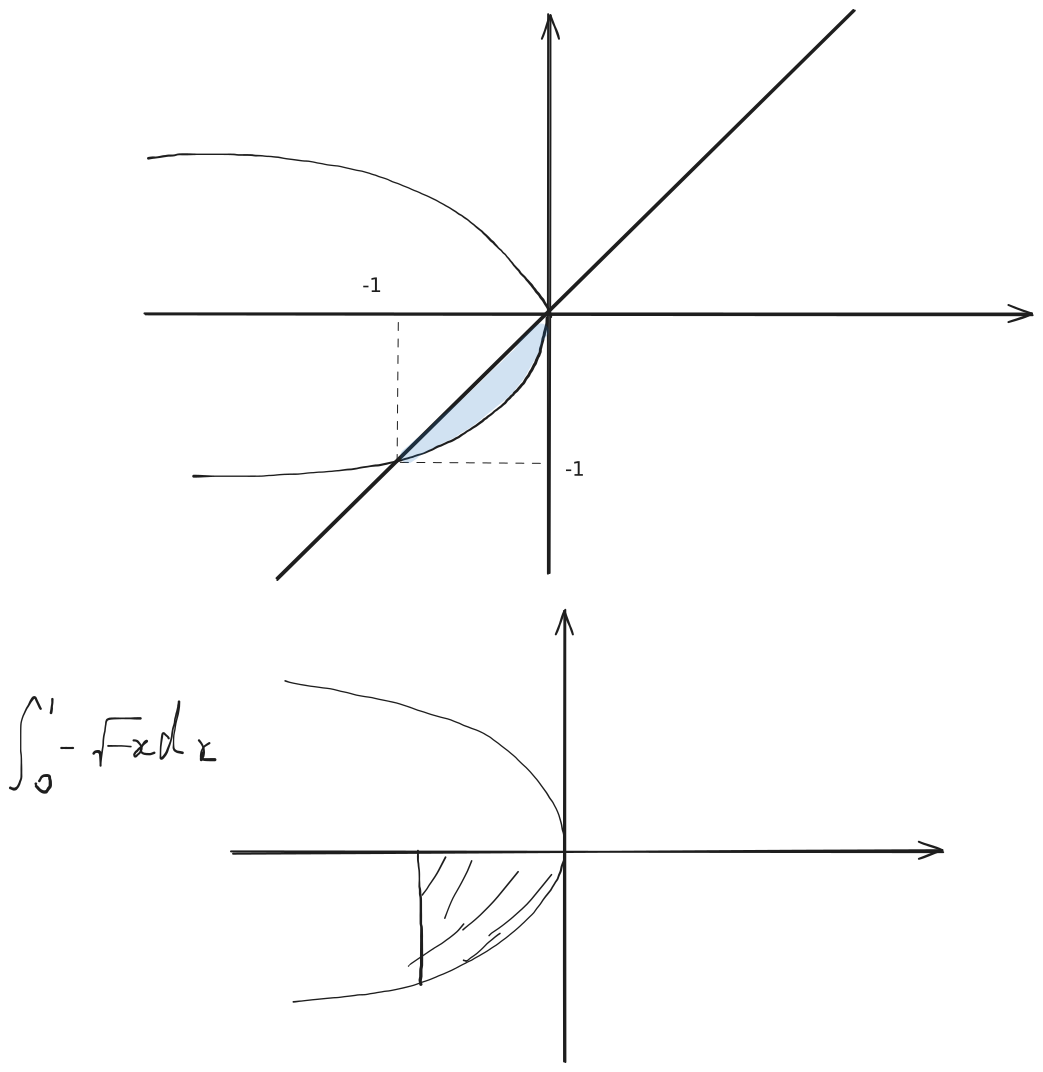
{ y 2 = − x ( y 2 ≥ 0 ) y = x x 2 = − x x 2 + x = 0 x ( 1 + x ) = 0 得到交点 ( 0 , 0 ) 和 ( − 1 , − 1 ) y 2 = − x ∴ y = − − x ,要曲线的下半枝 A = ∫ a b [ f u pp er ( x ) − f l o w er ( x )] d x A = ∫ − 1 0 [ x − ( − − x )] d x = 6 1 用Y形图做
{ y 2 = − x ( y 2 ≥ 0 ) y = x ⇒ { x = − y 2 x = y ∫ c d f 右 ( y ) − f 左 ( y ) d y S = ∫ − 1 0 − y 2 d y − ∫ − 1 0 y d y = − 3 1 y 3 − 1 0 − 2 1 y 2 − 1 0 = − ( 0 − 3 1 ⋅ ( − 1 ) ) − ( 0 − 2 1 ) = − 3 1 + 2 1 = − 6 2 + 6 3 = 6 1 求曲线x = y 2 , y = x − 2
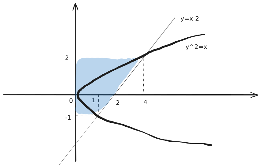
y 2 = x ,开口向右 { y 2 = x y = x − 2 交点 ( 1 , − 1 ) 和 ( 4 , 2 )
{ x = y 2 x = y + 2 ∫ − 1 2 ( y + 2 − y 2 ) d y 用X型图做
y 2 = x { y = + x 上支 y = − x 下支 与 y = x − 2 ∫ 0 1 [ x − ( − x )] d x + ∫ 1 4 [ x − ( x − 2 )] d x 求椭圆面积
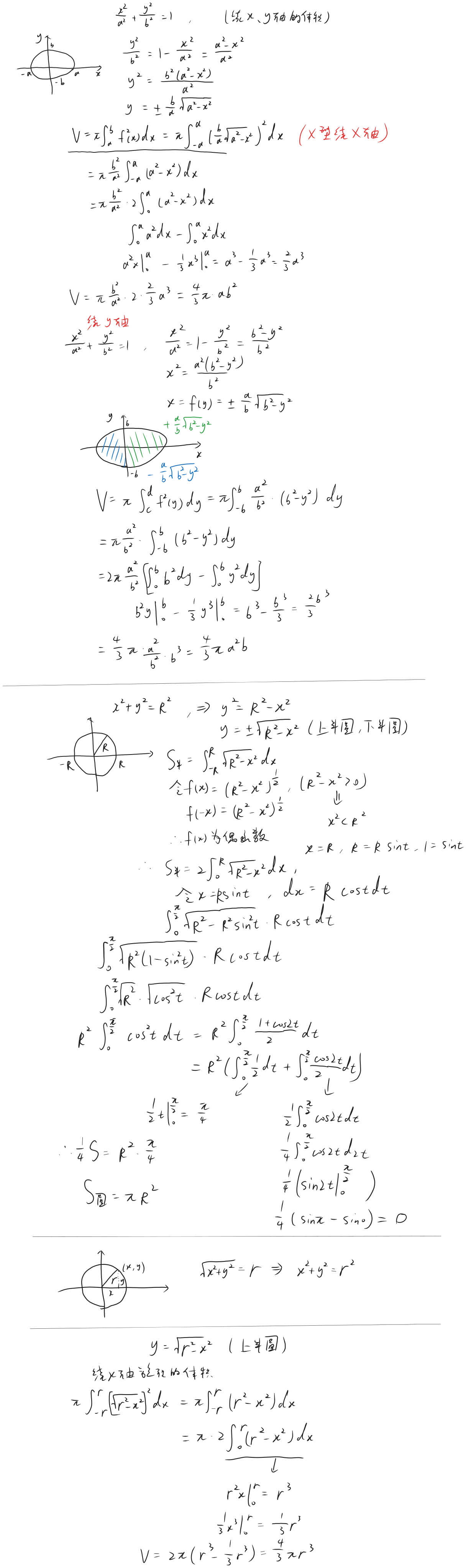
求椭圆a 2 x 2 + b 2 y 2 = 1
S = 4 S 1 = 4 ∫ 0 a y d x 利用椭圆的参数方程
{ x = a cos t y = b sin t 用定积分换元法
d x = d ( a cos t ) = a ⋅ ( − sin t ) d t = − a sin t d t x = 0 时 , t = 2 π x = a 时 , t = 0 ∴ S = 4 ∫ 2 π 0 b sin t ( − a sin t ) d t = 4 ∫ 0 2 π ab sin 2 t d t = 4 ab ∫ 0 2 π 2 1 − cos 2 t d t = 4 ab ( ∫ 0 2 π 2 1 d t − 2 1 ∫ 0 2 π cos 2 t d t ) = 4 ab ( ∫ 0 2 π 2 1 d t − 4 1 ∫ 0 2 π cos 2 t d ( 2 t ) ) = 4 ab [ 2 1 t 0 2 π − 4 1 ( sin 2 t ) 0 2 π ] = 4 ab ( 4 π − 4 1 ⋅ 0 ) = abπ = πab 另一种方法
a 2 x 2 + b 2 y 2 = 1 b 2 y 2 = 1 − a 2 x 2 y 2 = b 2 ( 1 − a 2 x 2 ) y 2 = b 2 ( a 2 a 2 − x 2 ) y 2 = a 2 b 2 ( a 2 − x 2 ) y = ± a 2 b 2 ( a 2 − x 2 ) = ± a b ( a 2 − x 2 ) y = a b ( a 2 − x 2 ) 为上半椭圆 y = − a b ( a 2 − x 2 ) 为下半椭圆 ∴ S = 4 ∫ 0 a a b ( a 2 − x 2 ) d x = 4 ⋅ a b ⋅ 4 1 π a 2 = πab 求弧长*
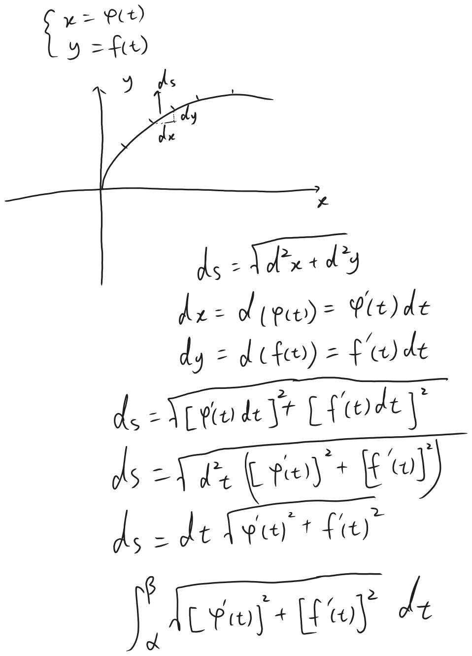
参数方程情形:
{ x = ϕ ( t ) y = f ( t ) α ≤ t ≤ β 且 ϕ ( t ) , f ( t ) 在 [ α , β ] 上一阶连续导数 = 0 S = ∫ α β [ φ ′ ( t ) ] 2 + [ f ′ ( t ) ] 2 d t 弧长公式的推导
{ y = f ( x ) x = x a ≤ x ≤ b ∴ S = ∫ a b [ f ′ ( x ) ] 2 + 1 2 d x S = ∫ a b 1 + [ f ′ ( x ) ] 2 d x 分段函数求定积分
∫ a b f ( x ) d x = ∫ a x 0 f ( x ) d x + ∫ x 0 b f ( x ) d x 其中x 0
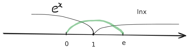
设f ( x ) = { e x , x ≤ 1 ln x , x > 1 ∫ 0 e f ( x ) d x
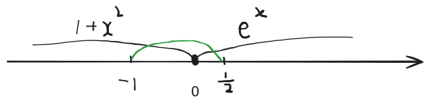
∫ 0 1 f ( x ) d x + ∫ 1 e f ( x ) d x ∫ 0 1 e x d x + ∫ 1 e ln x d x e x 0 1 + ( ln x ⋅ x ) 1 e − ∫ 1 e x ⋅ x 1 d x e − 1 + e − ∫ 1 e 1 d x 2 e − 1 − ( e − 1 ) = e 设f ( x ) = { 1 + x 2 , x < 0 e x , x ≥ 0 ∫ 2 1 2 f ( 1 − x ) d x
令 1 − x = t , x = 1 − t , d x = − d t 换元上下限,代入式子 1 − x = t x = 2 1 , t = 1 − 2 1 = 2 1 x = 2 , t = 1 − 2 = − 1 ∴ ∫ 2 1 2 f ( 1 − x ) d x = − ∫ 2 1 − 1 f ( t ) d t = ∫ − 1 2 1 f ( t ) d t = ∫ − 1 2 1 f ( x ) d x
∫ − 1 0 f ( x ) d x + ∫ 0 2 1 f ( x ) d x ∫ − 1 0 ( 1 + x 2 ) d x + ∫ 0 2 1 e x d x ( x + 3 1 x 3 ) − 1 0 + e x 0 2 1 = − ( − 1 − 3 1 ) + e 2 1 − 1 = 1 + 3 1 − 1 + e 2 1 = 3 1 + e 2 1 定积分等式证明
区间再现公式
积分区间再现公式
∫ a b f ( x ) d x = ∫ a b f ( a + b − x ) d x 证明
令 a + b − x = t , x = a + b − t d x = d ( a + b − t ) = − d t 当 x = a 时, t = b 当 x = b 时, t = a 故原式 = − ∫ b a f ( t ) d t = ∫ a b f ( t ) d t = ∫ a b f ( x ) d x 使用条件:等式两侧,积分区间一样
∫ a b f ( x ) d x = ∫ a b f ( a + b − x ) d x = 2 1 ∫ a b [ f ( x ) + f ( a + b − x )] d x 证明:
∫ 0 1 x m ( 1 − x ) n d x = ∫ 0 1 x n ( 1 − x ) m d x ∵ ∫ a b f ( x ) d x = ∫ a b f ( a + b − x ) d x 自变量 x 变为 ( 上限 + 下限 − x ) ∫ 0 1 x m ( 1 − x ) n d x = ∫ 0 1 ( 1 + 0 − x ) m [ 1 − ( 1 + 0 − x ) ] n = ∫ 0 1 ( 1 − x ) m ( x ) n 故原式成立 证明
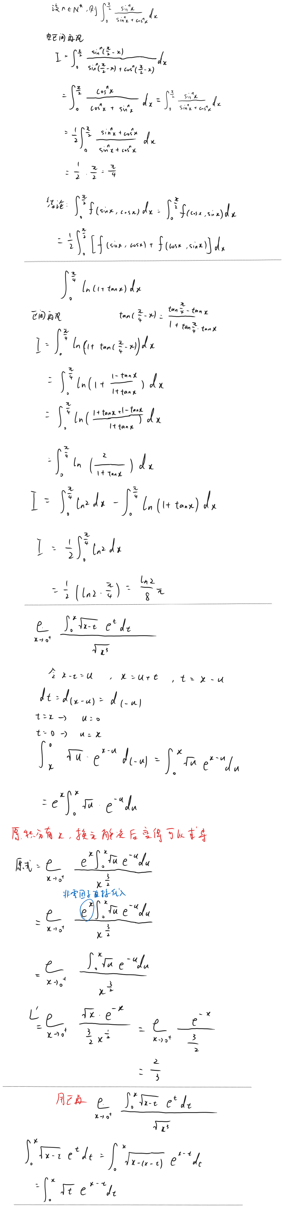
∫ 0 2 π f ( sin x ) d x = ∫ 0 2 π f ( cos x ) d x 第一种方法用上面的公式 ∵ ∫ a b f ( x ) d x = ∫ a b f ( a + b − x ) d x ∴ ∫ 0 2 π f ( sin x ) d x = ∫ 0 2 π sin ( 2 π − x ) d x = ∫ 0 2 π cos x d x 故原式成立 第二种方法,令 x = 2 π − t , d x = d ( 2 π − t ) = − d t 当 x = 0 , t = 2 π 当 x = 2 π , t = 0 ∴ ∫ 0 2 π f ( sin x ) d x = − ∫ 2 π 0 f [ sin ( 2 π − t ) ] d t = ∫ 0 2 π f ( cos t ) d t = ∫ 0 2 π f ( cos x ) d x 故原式成立 证明∫ 0 π x ⋅ f ( sin x ) d x = 2 π ∫ 0 π f ( sin x ) d x
∵ ∫ a b f ( x ) d x ∫ 0 π x ⋅ f ( sin x ) d x = = ∴ ∫ 0 π x ⋅ f ( sin x ) d x ∴ = ∫ a b f ( a + b − x ) d x = ∫ 0 π ( π − x ) ⋅ f ( sin ( π − x )) d x ∫ 0 π ( π − x ) ⋅ f ( sin x ) d x ∫ 0 π π ⋅ f ( sin x ) d x − ∫ 0 π x ⋅ f ( sin x ) d x = ∫ 0 π π ⋅ f ( sin x ) d x − ∫ 0 π x ⋅ f ( sin x ) d x 2 ∫ 0 π x ⋅ f ( sin x ) d x = ∫ 0 π π ⋅ f ( sin x ) d x 2 ∫ 0 π x ⋅ f ( sin x ) d x = π ∫ 0 π f ( sin x ) d x ∫ 0 π x ⋅ f ( sin x ) d x = 2 π ∫ 0 π f ( sin x ) d x 证明:
∫ 0 2 π sin x + cos x sin 3 x d x = ∫ 0 2 π sin x + cos x cos 3 x d x 并利用证明结果求∫ 0 2 π s i n x + c o s x s i n 3 x d x
∵ ∫ a a f ( x ) d x = ∫ a b f ( a + b − x ) d x ∫ 0 2 π sin x + cos x sin 3 x d x = ∫ 0 2 π sin ( 2 π − x ) + cos ( 2 π − x ) sin 3 ( 2 π − x ) d x = ∫ 0 2 π cos x + sin x cos 3 x d x 故原式得证 2 ∫ 0 2 π sin x + cos x sin 3 x d x = ∫ 0 2 π sin x + cos x sin 3 x d x + ∫ 0 2 π sin x + cos x cos 3 x d x 2 ∫ 0 2 π sin x + cos x sin 3 x d x = ∫ 0 2 π sin x + cos x sin 3 x + cos 3 x d x ∴ ∫ 0 2 π sin x + cos x sin 3 x d x = 2 1 ∫ 0 2 π sin x + cos x sin 3 x + cos 3 x d x 用立方和公式
( a + b ) 3 = a 3 + 3 a 2 b + 3 a b 2 + b 3 ( a − b ) 3 = a 3 − 3 a 2 b + 3 a b 2 − b 3 a 3 + b 3 = ( a + b ) ( a 2 − ab + b 2 ) a 3 − b 3 = ( a − b ) ( a 2 + ab + b 2 ) sin x + cos x sin 3 x + cos 3 x = sin x + cos x ( sin x + cos ) ( sin 2 x − sin x cos + cos 2 x ) = sin 2 x − sin x cos + cos 2 x = 1 − sin x cos x ∴ ∫ 0 2 π sin x + cos x sin 3 x d x = 2 1 ∫ 0 2 π ( 1 − sin x cos x ) d x 2 1 ( ∫ 0 2 π 1 d x − ∫ 0 2 π sin x d ( sin x ) ) 令 sin x = u x = 2 π , u = 1 x = 0 , u = 0 2 1 ( 2 π − ∫ 0 1 u d u ) 4 π − 2 1 ⋅ ( 2 1 ⋅ u 2 ) 0 1 = 4 π − 2 1 ( 2 1 ) = 4 π − 1 证明:F ( x ) = ∫ 0 π ln ( x 2 + 2 x cos t + 1 ) d t
欲证 F ( x ) 为偶函数 则 F ( x ) = F ( − x ) F ( − x ) = ∫ 0 π ln ( x 2 − 2 x cos t + 1 ) d t 又 ∵ ∫ a b f ( x ) d x = ∫ a b f ( a + b − x ) d x ∴ ∫ 0 π ln ( x 2 − 2 x cos t + 1 ) d t = ∫ 0 π ln ( x 2 − 2 x cos ( π − t ) + 1 ) d t = ∫ 0 π ln ( x 2 − 2 x ⋅ ( − cos t ) + 1 ) d t = ∫ 0 π ln ( x 2 + 2 x cos t + 1 ) d t = F ( x ) ∴ F ( x ) = F ( − x ) 求数列极限
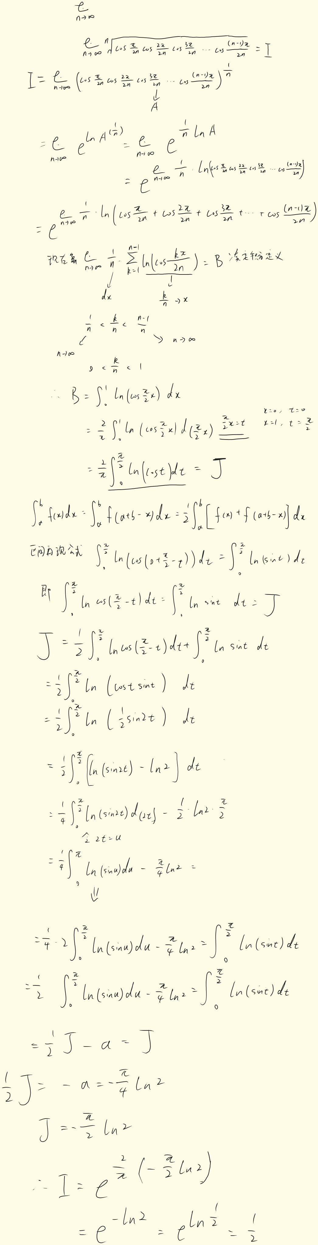
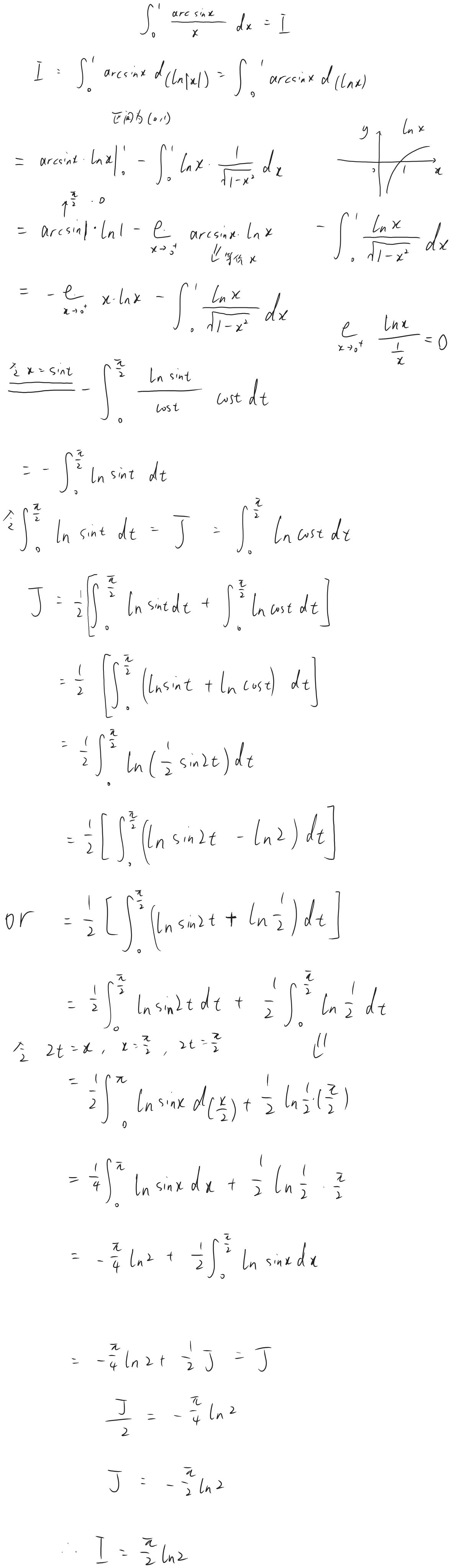
π 2 ∫ 0 2 π ln ( cos t ) d t 令 ∫ 0 2 π ln ( cos t ) d t = J 区间再现 J = ∫ 0 2 π ln ( cos t ) d t = ∫ 0 2 π ln ( sin t ) d t J = 2 1 ∫ 0 2 π ln ( sin t ) d t + ∫ 0 2 π ln ( cos t ) d t J = 2 1 ∫ 0 2 π ln ( sin t cos t ) d t J = 2 1 ∫ 0 2 π ln ( 2 1 sin 2 t ) d t J = 2 1 ∫ 0 2 π ln ( 2 sin 2 t ) d t J = 2 1 ∫ 0 2 π sin 2 t d t − 2 1 ∫ 0 2 π ln 2 d t J = 4 1 ∫ 0 π sin u d u − 2 1 ⋅ 2 π ⋅ ln 2 J = 2 1 J − 4 π ln 2 J = − 2 π ln 2
The interval reappearance formula
广义积分
又叫反常积分
无穷积分
也就是在无穷区间上的反常积分。上下界有一个是无穷,或都为无穷。∫ a + ∞ f ( x ) d x = lim t → ∞ ∫ a t f ( x ) d x = lim t → ∞ [ F ( t ) − F ( a )] ∫ a + ∞ f ( x ) d x
∫ a + ∞ f ( x ) d x = F ( x ) a + ∞ = F ( + ∞ ) − F ( a ) 比如:
∫ 0 + ∞ 1 + x 2 1 d x = arctan x 0 + ∞ = x → + ∞ lim arctan x − arctan 0 = 2 π ∴ ∫ 0 + ∞ 1 + x 2 1 d x 收敛 注意:∫ − ∞ + ∞ f ( x ) d x ∫ − ∞ a f ( x ) d x + ∫ a + ∞ f ( x ) d x ∫ − ∞ + ∞ f ( x ) d x
( − ∞ , + ∞ ) ∫ − ∞ + ∞ f ( x ) d x ∫ − ∞ a f ( x ) d x ∫ a + ∞ f ( x ) d x
∫ − ∞ + ∞ x d x = ∫ − ∞ 0 x d x + ∫ 0 + ∞ x d x = 2 1 x 2 − ∞ 0 + 2 1 x 2 0 + ∞ 其中 2 1 x 2 − ∞ 0 为 − ∞ 2 1 x 2 0 + ∞ 为 + ∞ 这两个极限都发散 所以原积分也发散 再举一个例子
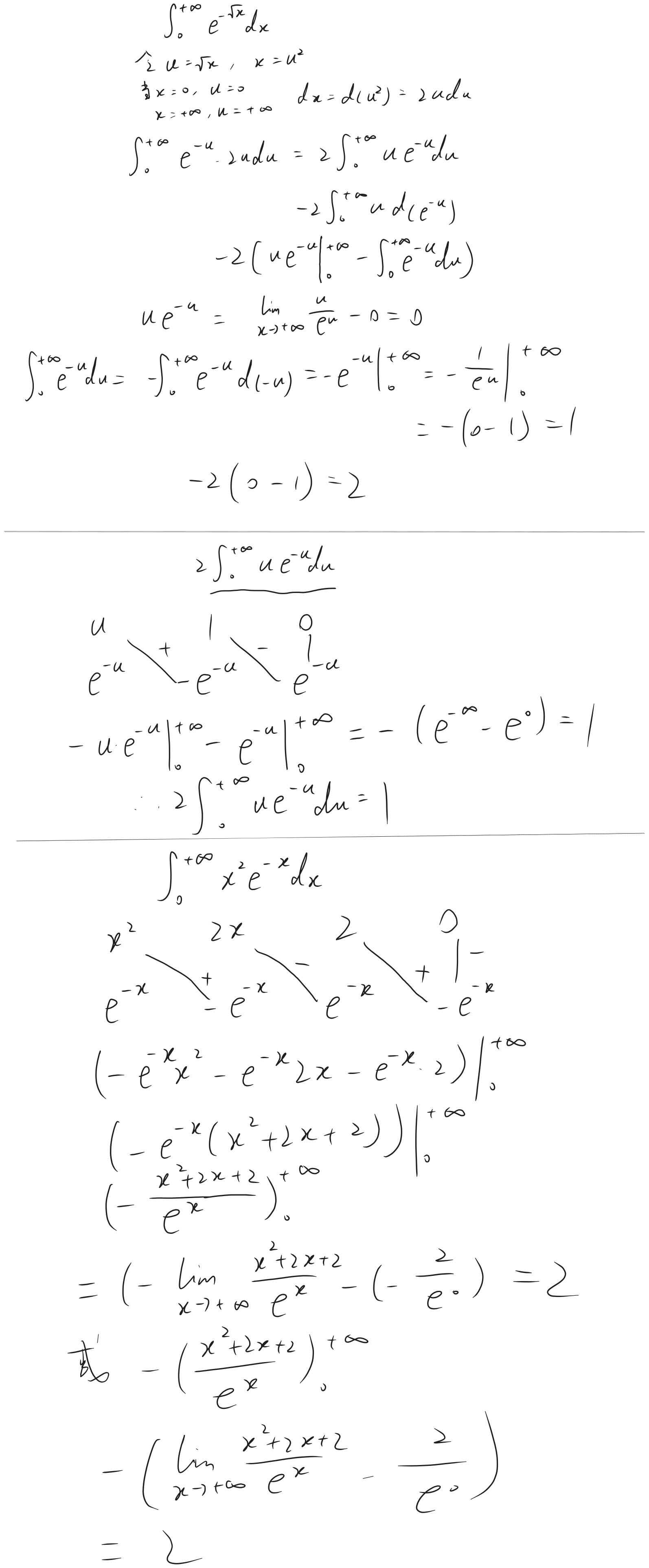
∫ − ∞ + ∞ x e − x 2 d x = ∫ 0 + ∞ x e − x 2 d x + ∫ − ∞ 0 x e − x 2 d x ∫ 0 + ∞ x e − x 2 d x = 2 1 ∫ 0 + ∞ e − x 2 d ( x 2 ) 令 x 2 = u = 2 1 ∫ 0 + ∞ e − u d u = − 2 1 ∫ 0 + ∞ e − u d ( − u ) = − 2 1 e − u 0 + ∞ = − 2 1 e − x 2 0 + ∞ − 2 1 ( x → + ∞ lim e − x 2 − 1 ) = 2 1 ∫ − ∞ 0 x e − x 2 d x = − 2 1 e − x 2 − ∞ 0 = − 2 1 ( 0 − x → − ∞ lim e − x 2 ) = − 2 1 拆开的两个积分都收敛,原积分可以用偶倍奇零e − x 2 ∫ − ∞ + ∞ x e − x 2 d x = 0
∫ − ∞ + ∞ e a x 2 P ( x ) d x , P ( x ) 为多项式 这类积分都都收敛,因为指数函数e x 2
∫ 1 + ∞ x 2 1 d x = − x 1 1 + ∞ = x → + ∞ lim − x 1 − ( − 1 1 ) = 0 + 1 = 1 ∫ 0 + ∞ x ⋅ e − 2 x d x − 2 1 ∫ 0 + ∞ x d ( e − 2 x ) d x − 2 1 [ ( x ⋅ e − 2 x ) 0 + ∞ − ∫ 0 + ∞ e − 2 x d x ] − 2 1 x e − 2 x 0 + ∞ + 2 1 ∫ 0 + ∞ e − 2 x d x − 2 1 x → + ∞ lim x ⋅ e 2 x 1 − 4 1 ∫ 0 + ∞ e − 2 x d ( − 2 x ) − 2 1 x → + ∞ lim e 2 x x − 4 1 ⋅ e − 2 x 0 + ∞ − x → + ∞ lim e 2 x 1 − 4 1 ⋅ ( e − ∞ − e 0 ) 0 − 4 1 ( 0 − 1 ) = 4 1 若∫ 0 + ∞ e k x d x = 2 1
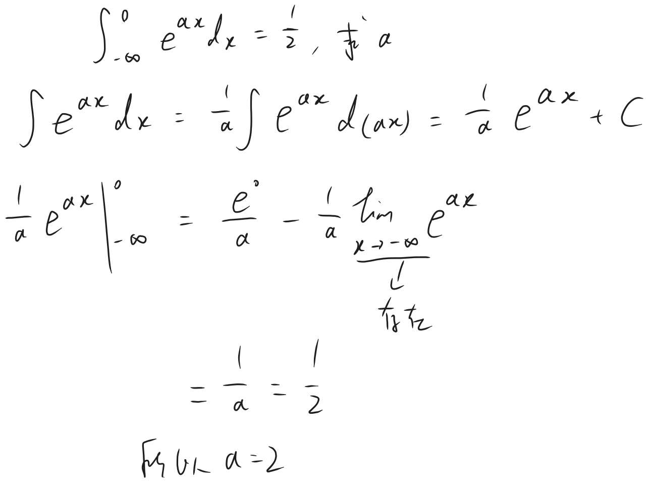
先算一下原函数 ∫ e k x d x = k 1 ∫ e k x d ( k x ) = k 1 ⋅ e k x + C ∫ 0 + ∞ e k x d x = k e k x 0 + ∞ x → + ∞ lim k e k x − k 1 如果 k > 0 , e k x → + ∞ 如果 k < 0 , e k x → 0 ∴ k < 0 x → + ∞ lim k e k x − k 1 = k 0 − 1 = − k 1 = 2 1 k = − 2 ∫ − ∞ + ∞ x 2 + 2 x + 2 1 d x ( x + 1 ) 2 = x 2 + 2 x + 1 ∫ − ∞ + ∞ ( x + 1 ) 2 + 1 1 d x ∫ − ∞ + ∞ ( x + 1 ) 2 + 1 1 d ( x + 1 ) 令 u = x + 1 ∫ − ∞ + ∞ 1 + u 2 1 d u = arctan u ∣ − ∞ + ∞ = x → + ∞ lim arctan x − x → − ∞ lim arctan x = 2 π − ( − 2 π ) = π
瑕积分
无界函数的反常积分
教材定义**(了解)**
设函数f(x)在(a,b]上连续,且lim x → a + = ∞ ϵ > 0 lim ϵ → 0 + ∫ a + ϵ b f ( x ) d x (a,b]上的广义积分,记作∫ a b f ( x ) d x ∫ a b f ( x ) d x = lim ϵ → 0 + ∫ a + ϵ b f ( x ) d x
Drawing 2026-01-14 16.56.42.excalidraw ⚠ Switch to EXCALIDRAW VIEW in the MORE OPTIONS menu of this document. ⚠ You can decompress Drawing data with the command palette: ‘Decompress current Excalidraw file’. For more info check in plugin settings under ‘Saving’
Excalidraw Data
Text Elements
a
b
Link to original
考研定义
设函数f(x)在(a,b]上连续,且lim x → a + f ( x ) = ∞
如∫ 0 1 x 1 d x lim x → 0 + x 1 = + ∞ ∫ 0 1 x 1 d x
设 a 为f(x)的瑕点(f ( x ) x = a ∫ a b f ( x ) d x = F ( x ) a + b = F ( b ) − F ( a + ) ∫ a b f ( x ) d x
Circular transclusion detected: Math/lib/Integral-libs/Drawing-2026-01-14-16.56.42.excalidraw
设 b 为f(x)的瑕点(f ( x ) x = b ∫ a b f ( x ) d x = F ( x ) a b − = F ( b − ) − F ( a ) ∫ a b f ( x ) d x
Drawing 2026-01-15 14.49.39.excalidraw ⚠ Switch to EXCALIDRAW VIEW in the MORE OPTIONS menu of this document. ⚠ You can decompress Drawing data with the command palette: ‘Decompress current Excalidraw file’. For more info check in plugin settings under ‘Saving’
Excalidraw Data
Text Elements
a
b
Link to original [a,b]内部,则f(x)在[a,b]上的广义积分为
∫ a b f ( x ) d x = ∫ a c f ( x ) d x + ∫ c b f ( x ) d x = F ( x ) ∣ a c + F ( x ) ∣ c b = [ F ( c − ) − F ( a )] + [ F ( b ) − F ( c + )] 做题步骤:
判断被积函数f(x)是否连续,用来排除瑕点在内部的情况(在内部就拆开)
按普通积分算
能代值则完毕,带入不了,就考虑极限
题目
∫ 0 1 x s i n x d x
x → 0 + lim x sin x = 1 ∴ x = 0 不是瑕点 ∫ 0 1 x 1 d x ∫ 0 1 x 1 d x = 2 x 0 1 = 2 − 0 = 2 为什么可以直接代值,这道题直接代值本质是算F ( x ) = 2 x 因为可以直接带入x=0,F(x)函数存在 ),所以极限值等于函数值,等于lim x → 0 + 2 x = 0
∫ − 1 1 x 2 1 d x x = 0 为瑕点 ∫ − 1 1 x 2 1 d x = ∫ − 1 0 x 2 1 d x + ∫ 0 1 x 2 1 d x − x 1 − 1 0 + ( − x 1 ) 0 1
-1 --- 0(瑕点) --- 1
− x 1 − 1 0 , − x 1 0 1 , − x 1 − 1 0 + ( − x 1 ) 0 1 = − x ∈ ( − 1 , 0 ) x ∈ ( 0 , 1 ) = x → 0 − lim ( − x 1 ) − ( − − 1 1 ) + ( − 1 1 − x → 0 + lim − ( x 1 ) ) ( − ∞ ) − 1 − 1 − ( − ∞ ) = + ∞ − 2 + ∞ = ∞ ∴ ∫ − 1 1 x 2 1 d x 发散 或者只算一个就行了
( − x 1 ) 0 1 = ( − 1 1 ) − x → 0 + lim ( − x 1 ) − 1 − ( − ∞ ) = + ∞ ∫ 0 1 x ln x d x x = 0 为瑕点 ∫ 0 1 ln x d ( ln x ) = 2 1 ln 2 x 0 1 = 2 1 ( ln 2 1 − x → 0 + lim ln 2 x ) x → 0 + , ln x → − ∞ , ln 2 x → + ∞ = 0 − 2 1 ⋅ ( + ∞ ) = − ∞ ∴ ∫ 0 1 x ln x d x 发散 这道题求完原函数,代入瑕点原函数的极限不存在,所以要取极限。
∫ 0 2 3 ( x − 1 ) 2 1 d x x = 1 为瑕点 ∫ 0 1 3 ( x − 1 ) 2 1 d x + ∫ 1 2 3 ( x − 1 ) 2 1 d x ∫ 0 1 ( x − 1 ) − 3 2 d ( x − 1 ) + ∫ 1 2 ( x − 1 ) − 3 2 d ( x − 1 ) 3 ( x − 1 ) 3 1 0 1 + 3 ( x − 1 ) 3 1 1 2 0 − 3 ( − 1 ) + 3 − 0 = 6 ∫ 0 2 4 − x 2 1 d x x=2为瑕点arcsin x
∫ 0 2 4 − x 2 1 d x = ∫ 0 2 4 ( 1 − 4 x 2 ) 1 d x 2 ∫ 0 2 1 − 4 x 2 1 d x 2 ∫ 0 2 1 − ( 2 x ) 2 1 d x ∫ 0 2 1 − ( 2 x ) 2 1 d ( 2 x ) arcsin 2 x 0 2 = arcsin 1 − arcsin 0 = 2 π 也可以用三角换元来做
∫ 0 2 4 − x 2 1 d x 令 x = 2 sin t , d x = d ( 2 sin t ) = 2 cos t d t x = 2 , 2 = 2 sin t , t = 2 π x = 0 , t = 0 4 − x 2 = 4 − 4 sin 2 t = 4 ( 1 − sin 2 t ) = 2 cos t ∫ 0 2 π 2 cos t 1 2 cos t d t = ∫ 0 2 π 1 d t = t 0 2 π = 2 π ∫ 0 1 1 − x 2 1 d x arcsin x 0 1 = x → 1 − lim arcsin x − arcsin 0 = 2 π arcsin x 0 1 = x → 1 lim arcsin x − arcsin 0 = 2 π arcsin x 0 1 = arcsin x − arcsin 0 = 2 π 这三种写法都可以
由于函数 f ( x ) = arcsin x [ − 1 , 1 ] x = 1 1 +
教材逻辑: 当一个函数在某点的某侧没有定义时,在该点处的极限 lim x → 1
∫ − 1 1 x 4 1 d x x → 0 lim x 4 1 = ∞ , x = 0 为瑕点 ∫ − 1 1 x 4 1 d x = ∫ − 1 0 x 4 1 d x + ∫ 0 1 x 4 1 d x ∫ − 1 0 x − 4 d x = − 3 1 x − 3 − 1 0 = − 3 1 ⋅ x 3 1 − 1 0 = − 3 1 ⋅ ( x → 0 − lim x 3 1 − 1 ) = ∞ ∴ ∫ − 1 1 x 4 1 d x 发散 ∫ 0 1 ln ( 1 − x ) d x 定义域: 1 − x > 0 , x < 1 x = 1 为瑕点 x ⋅ ln ( 1 − x ) 0 1 + ∫ 0 1 x ⋅ 1 − x 1 d x 先求一下积分原函数 ∫ 0 1 1 − x x d x = − ∫ 0 1 1 − x ( 1 − x ) − 1 d x = − [ ∫ 0 1 d x − ∫ 0 1 1 − x 1 d x ] = − ( 1 + ∫ 0 1 1 − x 1 d ( 1 − x ) ) = − 1 − ln ∣1 − x ∣ 0 1 = − 1 − ln ( 1 − x ) 0 1 = − 1 − lim x → 1 − ln ( 1 − x ) x ⋅ ln ( 1 − x ) 0 1 = lim x → 1 − x ⋅ ln ( 1 − x ) lim x → 1 − x ⋅ ln ( 1 − x ) − lim x → 1 − ln ( 1 − x ) − 1 合并 lim x → 1 − x ⋅ ln ( 1 − x ) − ln ( 1 − x ) − 1 lim x → 1 − ( x − 1 ) ln ( 1 − x ) − 1 = − 1 为啥这里可以合并?
这里极限可以直接合并,因为本质是求 ∫ ln ( 1 − x ) d x ∫ ln ( 1 − x ) d x = x ln x + ∫ 1 − x x d x = x ln ( 1 − x ) − ∫ 1 − x ( 1 − x ) − 1 d x = x ln ( 1 − x ) − ∫ d x + ∫ 1 − x 1 d x = x ln ( 1 − x ) − ∫ d x − ∫ 1 − x 1 d ( 1 − x ) = x ln ( 1 − x ) − ln ∣1 − x ∣ − x + C [ x ln ( 1 − x ) − ln ∣1 − x ∣ − x ] 0 1 [ x ln ( 1 − x ) − ln ( 1 − x ) − x ] 0 1 [( x − 1 ) ln ( 1 − x ) − x ] 0 1 x → 1 − lim ( x − 1 ) ln ( 1 − x ) − x → 1 − lim x = − 1 另一种解法
∫ 0 1 ln ( 1 − x ) d x 令 t = 1 − x , x = 1 − t , d x = d ( 1 − t ) = − d t x = 1 , t = 0 x = 0 , t = 1 − ∫ 1 0 ln t d t = ∫ 0 1 ln t d t = ( t ln t 0 1 − ∫ 0 1 d t ) − t ln t 0 1 − 1 − ( 0 − x → 0 + lim t 1 ln t ) − 1 x → 0 + lim − t 2 1 t 1 = − x → 0 + lim t 1 ⋅ t 2 = x → 0 + lim t = 0 ∴ ∫ 0 1 ln ( 1 − x ) d x = − 1 常见结论
无穷区间积分
∫ a + ∞ x α ln β x d x ∫ a + ∞ x p 1 d x { p > 1 , p ≤ 1 , 收敛 发散 ( a > 0 ) ∫ a b ( x − a ) q d x , ∫ a b ( b − x ) q d x ⎩ ⎨ ⎧ q < 1 , 收敛 q ≥ 1 , 发散 = ⎩ ⎨ ⎧ α > 1 , 收敛 , α < 1 , 发散 , α = 1 , { β > 1 , 收敛 , β ≤ 1 , 发散 . 积分下限 ( a > 1 ) 求旋转体体积
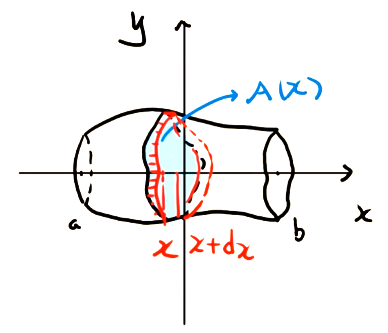
平行截面面积 已知立体体积的求法(理解)
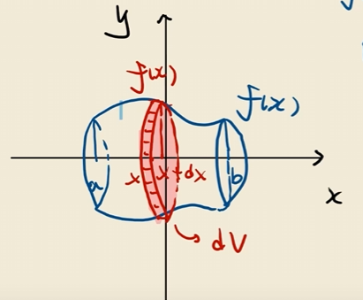
X型图绕X轴旋转
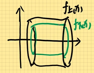
V = ∫ a b d V = ∫ a b π f 2 ( x ) d x = π ∫ a b f 2 ( x ) d x 若是两个函数f 上 ( x ) , f 下 ( x ) 间 的体积
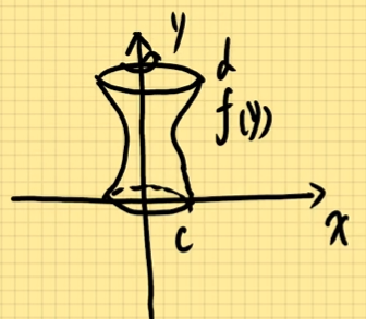
V = π ∫ a b f 上 2 ( x ) d x − π ∫ a b f 下 2 ( x ) d x Y型图绕Y轴旋转
V = π ∫ c d f 2 ( y ) d y 如果内部有嵌套
V = π ∫ c d [ f 右 2 ( y ) − f 左 2 ( y )] d y X型图绕Y轴旋转
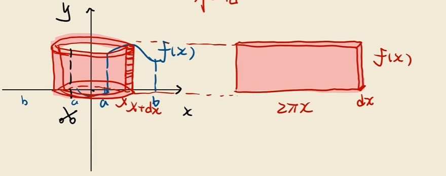
V = ∫ a b 2 π x ⋅ f ( x ) d x = 2 π ∫ a b x f ( x ) d x 题目
求由y = sin x , 0 ≤ x ≤ π
Drawing 2026-01-23 15.23.27.excalidraw ⚠ Switch to EXCALIDRAW VIEW in the MORE OPTIONS menu of this document. ⚠ You can decompress Drawing data with the command palette: ‘Decompress current Excalidraw file’. For more info check in plugin settings under ‘Saving’
Excalidraw Data
Text Elements Link to original
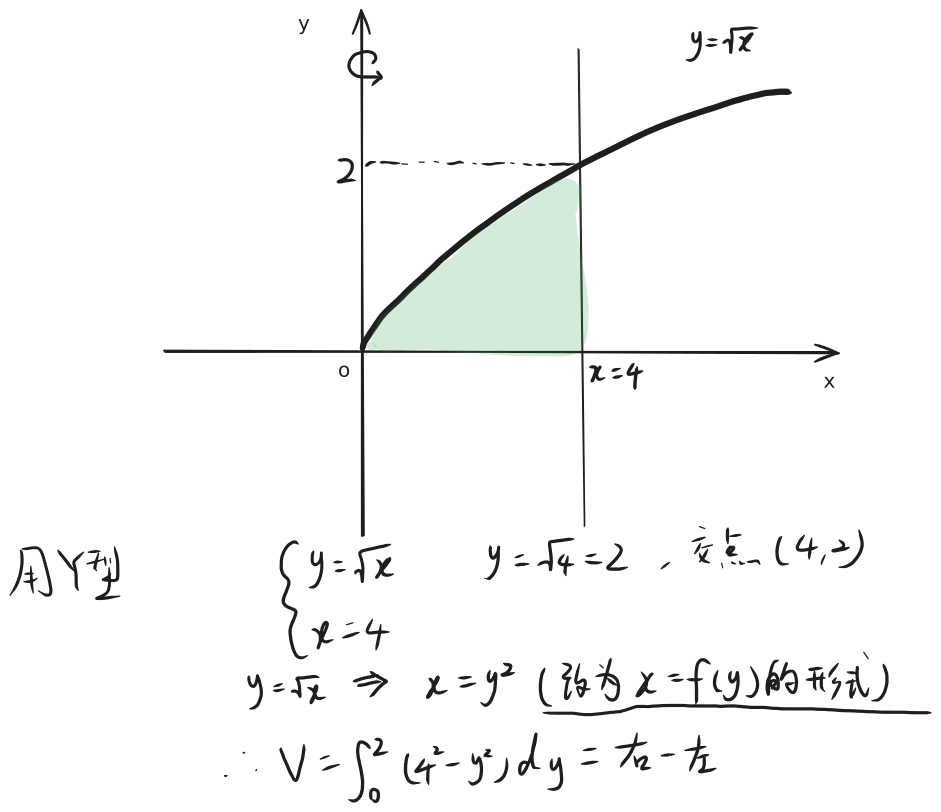
V = ∫ 0 π 2 π x ⋅ sin x d x = − 2 π ∫ 0 π x d ( cos x ) = − 2 π ( x cos 0 π − ∫ 0 π cos x d x ) = − 2 π ( π cos π − sin π ) = − 2 π ( − π ) = 2 π 2 求y = x , x = 4
{ y = x x = 4 交点 ( 4 , 2 ) 先求面积
Drawing 2026-01-23 15.45.49.excalidraw ⚠ Switch to EXCALIDRAW VIEW in the MORE OPTIONS menu of this document. ⚠ You can decompress Drawing data with the command palette: ‘Decompress current Excalidraw file’. For more info check in plugin settings under ‘Saving’
Excalidraw Data
Text Elements
4
2
x
0
Link to original
∫ 0 4 x d x = 3 16 另一种方式,用 Y 型图 y = x ⇒ x = y 2 { x = y 2 x = 4 ∫ 0 2 ( 4 − y 2 ) d y = 4 y 0 2 − 3 1 y 3 0 2 = 8 − 3 8 3 24 − 3 8 = 3 16 绕y轴的旋转体体积:
V = ∫ a b 2 π x ⋅ f ( x ) d x = 2 π ∫ 0 4 ( x ⋅ x ) d x 第二种方法套Y型图绕Y轴旋转的公式,做两个体积之差。
欧拉积分
Use the parity of the function to compute the definite integral
Drawing 2026-03-12 12.43.45.excalidraw ⚠ Switch to EXCALIDRAW VIEW in the MORE OPTIONS menu of this document. ⚠ You can decompress Drawing data with the command palette: ‘Decompress current Excalidraw file’. For more info check in plugin settings under ‘Saving’
Excalidraw Data
Text Elements Link to original
∫ 0 100 π ∣ sin x ∣ d x I = 100 ∫ 0 π sin x d x = 100 ⋅ ( − cos x ) 0 π = 100 ⋅ ( − cos π − ( − cos 0 )) = 100 ⋅ ( − ( − 1 ) − ( − 1 )) = 100 ⋅ ( 2 ) = 200 若f(x)的周期为T,
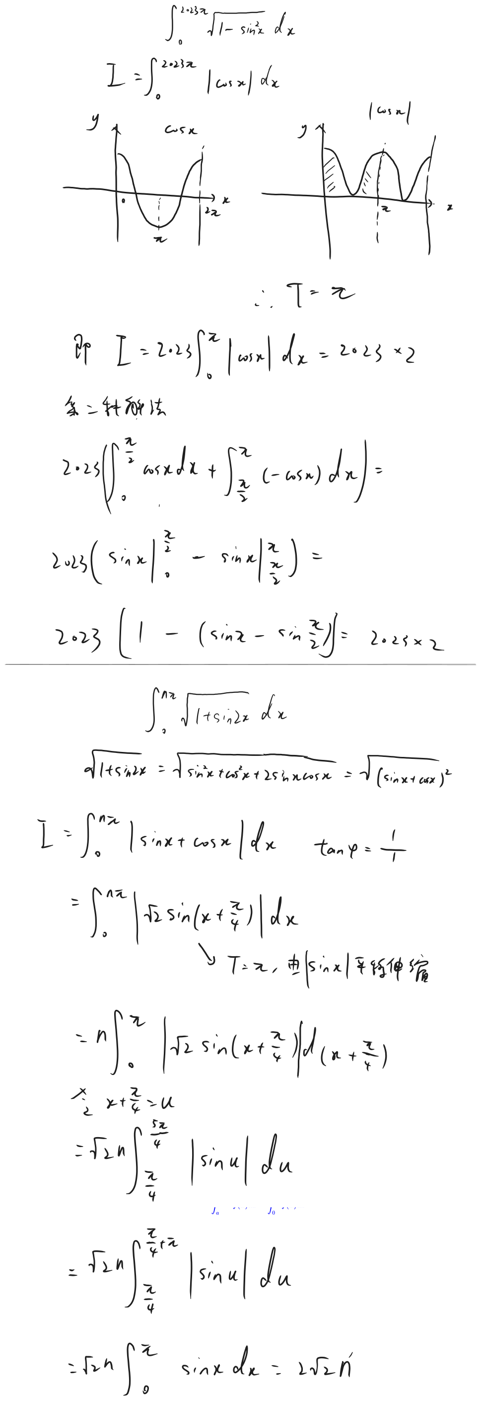
∫ 0 n T f ( x ) d x = n ∫ 0 T f ( x ) d x ∫ 0 2023 π 1 − cos 2 x d x ∫ 0 2023 π ∣ sin x ∣ d x f ( x ) 的周期 T = π ∴ I = 2023 ∫ 0 π sin x d x = 4046
设f(x)是以T为周期的连续函数,即f ( x + T ) = f ( x ) ∫ a a + T f ( x ) d x = ∫ 0 T f ( x ) d x
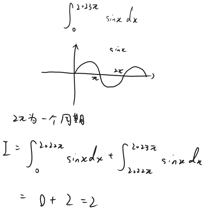
∫ 2 2 + π ∣ sin x ∣ d x = ∫ 0 π ∣ sin x ∣ d x ∫ 2022 π 2022 π + π sin x d x = ∫ 0 π sin x d x = 2 ∫ 2 2 + 5 π sin x d x = ∫ 0 5 π sin x d x = ∫ 0 4 π sin x d x + ∫ 4 π 5 π sin x d x = 2 ∫ 0 2 π sin x d x + ∫ 0 π sin x d x = 0 + 2 = 2 注,辅助角公式:
A sin α + B cos α = A 2 + B 2 sin ( α + φ ) 其中 tan φ = A B